Scrubbing Reads for Better Assembly

In an earlier post, I introduced the concept of  intrinsic quality values — a statistic indicating the quality of every say TP=100bp interval of a read — that could be computed from the pile of local alignments for each read computed by daligner with the -t option set to TP.  This idea is important because of the complex and variable error profile of PacBio long reads which I illustrated with the following hypothetical example:

Error profile of a typical long read. The average error rate is say 12% but it varies and occasionally is pure junk.

The quality values together with the pattern of alignments in a read’s pile allow one to detect these, sometimes long, low-quality segments of a read, as well as detect when the read is a chimer or contains undetected adaptamer sequence that should have been excised.  These artifacts are quite frequent in PacBio data sets and apart from repeats are the major cause of poor assembly.  We call the process of repairing the low-quality sequence and removing the chimers and missed adaptamers, scrubbing, and formally the goal of a scrubber is to edit a set of reads with as little loss of data as possible so that:

1. every edited read is a contiguous segment of the underlying genome being sequenced, and
2. every portion of a read is of reasonable quality, i.e. <20% error or Q8.

The conditions above are exactly those assumed by a string graph construction algorithm and any data that doesn’t meet these conditions introduces breaks and false branches in the string graph.  For this reason I choose to scrub hard, i.e. my scrubber will over call chimers and adaptamers rather than miss them, so that condition 1 above is meet by all the data after scrubbing.

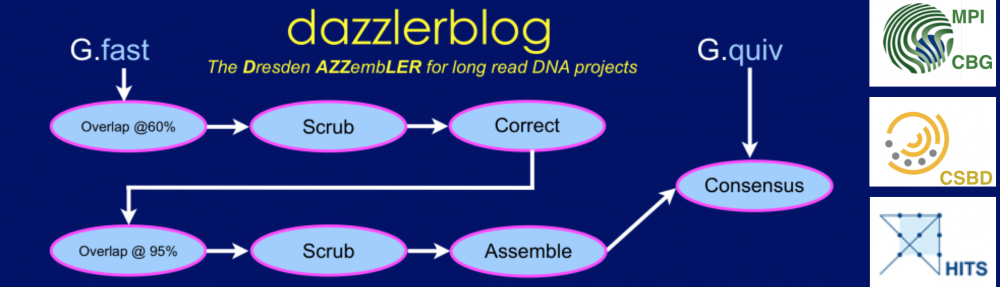
The scrubber module consists of a pipeline of 4-5 modules as opposed to a single program that performs the end-to-end task.  We structured it this way so that one can run each pass in a block-parallel manner on an HPC cluster, and secondarily, so that a creative user can potentially customize or improve aspects of the overall process.  The figure below, shows the pipeline:

Data flow, including tracks, of the scrubbing pipeline

Each program in the pipeline can be run on the overlap piles for a block of the underlying DB in parallel, allowing a simple HPC parallel scheme.  By doing so each program per force outputs only the portion of a track for the intput block (i.e.. .qual, .trim, .patch), and these block tracks must be concatenated into a single track for the entire database with Catrack before the next step in the pipeline can be performed.  Fortunately, this serial step is very fast, basically amounting to concatenating a number of files of total size O(R) where R is the number of reads in the database.

The first step in scrubbing is to compute the quality values for every read segment and record them in a qual track with DASqv as described in an earlier post.  Recall that with the -v option DASqv displays a histogram of the QV’s over the dataset.  Using this histogram one should select a threshold GOOD for which 80% of the QV’s are not greater than this value, and another BAD for which 5-7% of the QV’s are not less than this value.  In the next two steps of the pipeline, QV’s ≤ GOOD will be considered “(definitley) good”, and QV’s ≥ BAD will be considered “(definitely) bad”.  Any QV’s between the two thresholds will be considered of unknown quality.   Decreasing these values, increases the amount of data that will be scrubbed away as not of sufficient quality, and increasing these thresholds retains more data but at a sacrifice in quality.  The percentile guidelines above represent good settings for typical PacBio data (that is about 80% of the data actually is good and 5% of it is actually crap).

The GOOD/BAD thresholds must be supplied as the -g and -b parameters to the next phase of the pipeline realized by DAStrim.  DAStrim first uses the quality values and the supplied -g and -b thresholds to determine a sequence of high-quality (HQ) segments for the A-read of each pile.  Formally, an HQ segment begins and ends with a good  trace point interval interval, contains no bad intervals, and is at least 400bp long.  Any intervals before the first HQ segment and after the last HQ segment, are clipped/trimmed from the beginning and end of the read, respectively.  The main task of DAStrim, is to then determine what to do with the gaps between the HQ segments of a read.  There are 4 cases:

1. The gap is completely covered/spanned by lots of local alignments with other reads – then the gap is simply low quality sequence and deemed LOW-Q. This is illustrated in the example at right by the leftmost low-quality gap.
2. The gap is not spanned by local alignments with other reads, but most of the local alignments to the left (X) and right (Y) of the gap are for the same B-read and the distance between the two B-read segments in the relevant local alignments are consistent with the size of the gap – then the gap is a (very) low quality (and often long) drop out in the A-read and the gap is deemed LOW-Q.
3. the gap is not spanned but the left (X) and right (Y) alignment sets have the relevant B-reads in the complement orientation with respect to each other – the gap is due to an ADAPTAMER. Typically, the gap is also very sharp with the gap between paired local alignments being very narrow as in the example below left.  In the situation where one or more adatamer gaps is found for a read, all but the longest subread between two of the adaptamers is thrown away.

   

4. the gap is not spanned and there is no correspondence between the reads in the local alignments to the left and right – the gap is due to a chimeric join in the A-read and the gap is designated CHIMER as illustrated in the example above right.  Every chimeric gap splits the A-read into two new reads.

DAStrim outputs a track (or track block) called trim that for each read encodes the begin/end coordinates for each HQ segment and the classification of each intervening gap (either LOW-Q or CHIMER).  With the -v option it also outputs a report describing how much data was trimmed, designated LOW-Q, etc.  In the example below, one sees that the left column is the number of reads or items, and the right column is the total number of bases in those items.  3,117 reads totalling 11.6% of the bases in the data set were found to be either garbage or were totally masked by the DAMASKER module and thrown out.  Of the remaining reads, 5.7% of the bases were trimmed from the beginning of reads, and 2.5% from the end of reads.  37 missed adaptamer sites were found and 117.8Kbp was trimmed away leaving only the longest sub-read between adaptamers.

Input:     22,403 (100.0%) reads      250,012,393 (100.0%) bases

Discard:    3,117 ( 13.9%) reads       29,036,136 ( 11.6%) bases
5' trim:   13,749 ( 61.4%) reads       14,137,800 (  5.7%) bases
3' trim:    7,919 ( 35.3%) reads        6,316,157 (  2.5%) bases
Adapter:       37 (  0.2%) reads          117,816 (  0.0%) bases

Gaps:      35,253 (157.4%) gaps        15,205,800 (  6.1%) bases
Low QV:    30,903 (137.9%) gaps         8,834,200 (  3.5%) bases
Span'd:     3,346 ( 14.9%) gaps         4,441,700 (  1.8%) bases
Chimer:     1,004 (  4.5%) gaps         1,929,900 (  0.8%) bases

Clipped:   25,826 clips                49,607,909 ( 20.6%) bases
Patched:   34,249 patches              13,275,900 (  5.3%) bases

In the adaptamer-free reads that were retained, there were 35,253 gaps between HQ segments.  30,903 were deemed LOW-Q by virtue of being spanned by alignments (Low QV) and 3,346 were deemed LOW-Q by virture of consistent alignment pairs (Span’d).  The remaining 1,004 where deemed to be CHIMERs and will be split creating 1,004 new reads.  The last two lines tell one that a total of 20.6% of the bases were lost altogether because of trimming, adapatmers, and chimers, and that 5.3% of the bases were in low-quality gaps that will be patched with better sequence in the ensuing scrubbing passes.

The 3rd phase of scrubbing is realized by DASpatch which selects a good B-read segment to replace each LOW-Q gap with.  We call this high-quality sequence a patch.  The program also reviews all the gap calls in light of the fact that the trimming of reads affects their B-read alignment intervals in the piles of other reads, occasionally implying that a gap should have been called a CHIMER and not LOW-Q.  DASpatch further changes a LOW-Q gap to a CHIMER call if it cannot find what it thinks is a good B-read segment to patch the gap.  The number of these calls is generally very small, often 0, and their number is reported when the -v option is set.  DASpatch outputs a track (or track block) called patch that encodes the sequence of B-read segments to use for patching each low quality gap in a read.

The final phase of scrubbing is to perform the patching/editing of reads that is encoded in the trim and patch tracks produced in the last two phases, and produce a new data base of all the resulting scrubbed reads.  This is accomplished by DASedit that takes the name of the original database and the name you would like for the new database as input.  This phase runs sequentially and can can be quite slow due to the random access pattern of read sequences required to patch, so you might want to go do something else while it runs.  But when its finished you will have a database of reads that are typically 99.99% chimer and adatamer free, and that contain almost no stretches of very low-quality base calls.

The new database does not have a .qvs or .arr component, that is it is a a sequence or S-database (see the original Dazzler DB post).  Very importantly, the new database has exactly the same block divisions as the original.  That is, all patched subreads in a block of the new database have been derived from reads of the same block in the original database, and only from those reads.  DASedit also produces a map track that for each read encodes the original read in the source DB that was patched and the segments of that read that were high-quality (i.e. not patched).  A program DASmap output this information in either an easy-to-read or an easy-to-parse format.  A small example of a snippet output by DASmap is as follows:

55 -> 57(2946) [400,2946]
56 -> 58(11256) [700,1900]
57 -> 58(11256) [6600,9900] 83 [10000,11256]
58 -> 59(12282) [400,4100] 88 [4200,9400] 97 [9500,12282]

The first line indicates that read 55 in the patched database was derived from read 57 in the original database and is the segment from [400,2946] of that read.  Reads 56 and 57 were both derived from read 58 in the original DB, and read 57 consists of segments [6600,9900] and [10000,11256] of read 58 with a patch between them of 83bp (but the source of the patch data is not given).  The read length of each original read is given for convenience.  The purpose of this map is to allow you to map back to the original reads in the final consensus phase of an assembly where one will want to use the original data along with its Quiver or Arrow data encoded in the .qvs/.arr component of the DB.

A database of scrubbed reads can be used in three ways as illustrated in the figure at the end of this paragraph.  In the first use-case, a user can simply take the database of scrubbed reads and use them as input to their favorite long-read assembler (e.g. Falcon or Canu).  In our experience doing so improves the assemblies produced by these third party systems.  For example, in the plot at right, Falcon’s error corrector (EC) tends to break reads at long low quality gaps producing the red line read-length profile given a data set with the blue read-length distribution.  When Falcon starts on our scrubbed reads with the grey read-length profile, (which is significantly better than the EC profile), its own error correct leaves these longer scrubbed reads intact. Longer reads into the string graph phase of Falcon’s assembler implies a more coherent assembly, i.e. longer contigs.The second use-case, is to rerun the daligner on this set of reads to produce .las files anew over the scrubbed reads.  The down side is that this takes considerable compute time.  However, because the reads are scrubbed, one should expect that reads properly overlap and a purely local alignments can now be ignored as repeat-induced.  Giving the result set of overlaps to a string graph algorithm for assembly should result in better assembly as many repeat-induced correspondences have been removed.

The final third use-case, is rather than re-run daligner, to take advantage of the fact that the piles computed the first time already contain all the pairs of reads that align, and so in fact all that needs to be done is to “re-align” an local alignment found between original reads in terms of the derived reads.  This includes extending the local alignment when the introduction of a patch allows it to now extend through a formerly low-quality region.  To this end I produced a program DASrealign that takes a pair of blocks of the scrubbed DB and the original .las file for the block pair (in the original DB), and produces the realigned overlap piles in a .las file for the scrubbed DB blocks.  Not carefully that this requires (1) that you have kept the block pair .las files produced by the first phase of the HPC.daligner process and not removed them, and (2) that after realigning every block pair, you must then merge these to produce the overlap blocks for the scrubbed DB.  This process is roughly 40x faster than running daligner from scratch.  The trade off is that some alignments might be missed that would otherwise be found if daligner were rerun on the scrubbed reads, and the trace point encoding of a patched alignment is no longer uniform in the A-read and so one could not scrub the patched reads a second time with the piles so produced.  On the otherhand, one can take just the overlaps that are produced this way and perform a string graph assembly.

The pipeline above careful identifies and removes read artifacts such as chimers and adapatamers, and repairs high error-rate read segments, providing a set of reads that will assemble well (without correction).  However, ultimately we believe good assembly will further require correction in order to carefully separate haplotypes and low copy number repeats prior to the string graph phase.  Therefore, our ultimate ongoing development plan is to replace DASedit with a program that produces error corrected A-reads based on the analysis of DASqv-DAStrim-DASpatch and to then realign (at much higher stringency / lower error rate) the resulting reads.  We expect this process to take more time than simply applying DASrealign, but with the advantage that the reads will also be error corrected.  Never the less, just scrubbing reads and feeding them into another assembler is proving to have sufficient value that I decided to release the current pipeline.  Best, Gene

Moving to the Sequel

In the last year, Pacbio has, in conjunction with the introduction of the Sequel instrument, made two changes to their software environment that affect downstream applications including the Dazzler suite.  Namely, they have (1) moved from the HDF5 format to the BAM format for the primary output of the instrument, and (2) there is a new alternative to the Quiver consensus base-caller, called Arrow that is equally if not more accurate and requires less information about the raw signal to do so.  Specifically, Quiver requires five quality streams each the length of the associated read, whereas Arrow needs more simply just the read’s pulse width stream clipped to the smallest four values and the four signal-to-noise (snr) ratios for each nucleotide channel.  All .bax.h5 files currently and previously produced for the RS II contain the the information needed by both Quiver and Arrow.  However, the new .subreads.bam files contain just the information needed by Arrow if they were produced by a Sequel instrument, but they can contain just the information needed by Quiver if it was produced by converting an RS II HDF5 file to a BAM file with the PacBio program bax2bam.

To accommodate these transitions, the Dazzler suite now interprets the .subreads.bam files produced by the instrument and can extract Quiver or Arrow information from either type of source file, and Dazzler DB’s have been upgraded to hold either the information needed by Quiver, or the information needed by Arrow (but not both).  Most of the new programs and modifications have occurred in the DEXTRACTOR module, although the upgrades also affected the DAZZ_DB module.  Below we outline the changes and new capabilities.

The original extraction program dextract can now also take a BAM file as input and from it produce a .fasta, a .quiva, an .arrow file, or some combination of these according to whether or not the command line options -f, -q, and -a, respectively, are set.  The .fasta and .quiva file types are unchanged, and the new .arrow file type contains the information needed by Arrow.  The dextract program has further been upgraded so that given an HDF5 file it too can produce any combination of the 3 files.  An example, of a sub-read entry in each format is immediately below and we explain the contents of each in the following paragraph.

A .fasta file is in FASTA format, and an entry consists of a standard “Pacbio header” followed by the DNA sequence on any number of ensuing lines.  The standard header contains the movie name, well number (44), pulse range (0-6289), and sequence quality value (.812) to 3 digits, always with the same syntax.  A .quiva file uses a FASTQ-like format, and an entry consists of the same Pacbio header, followed by each of the 5 quality streams, one per line, with no line breaks within a stream.  Finally, the .arrow file is in FASTA format, and an entry consists of a header with the movie name and the 4 snr values, followed by the pulse width stream on any number of ensuing lines.  The header in this case contains just the movie name and the four snr values (6.69, 5.89, 3.72, 4.04) in  a fixed syntax where the snr values are always to 2 digits of precision and always listed in the order of the A, C, G, and T channels, respectively.  The pulse width stream is always a sequence of the symbols, 1, 2, 3, and 4.

One might further recall that the DEXTRACTOR module also contains compression and decompression program pairs — dexta/undexta and dexqv/undexqv — that operate on .fasta and .quiva files, respectively.  There is now also a compressor/decompressor pair, dexar/undexar, that compresses an .arrow file into a .dexar file and decompresses it back.  The picture immediately below shows the existing programs in green and the new ones in orange:The numbers in green in the picture above give the approximate sizes of the various files in bytes, where N is the number of base pairs of data in the file.  The .bam file occupies roughly 2N bytes if it contains only Arrow information and 3.3N if it contains only Quiver information.  The larger bax.h5 file always contains the information for both programs within it.  The main thing to note is that the compressed files represent a significant space savings, but by not as big a margin over the .bam source files which are themselves gzip compressed.

Previously, a Dazzler DB held the DNA sequence and header information for each subread, and optionally could store and organize all the Quiver information.  I have upgraded the system so that now a DB can also optionally hold all the Arrow information for a project.  But note carefully, that a Dazzler DB cannot hold both.  So we term a DB that holds Quiver information a Quiver-DB (Q-DB), one that holds Arrow information an Arrow-DB (A-DB), and one that holds neither a Sequence-DB (S-DB).  One might think this forces a user to choose between Quiver and Arrow for consensus at the beginning of an assembly project, but this is not the case as one can at any time add or delete the Quiver or Arrow information independently of the sequence information.

Specifically, recall that one creates an S-DB, possibly incrementally, by adding .fasta files with fast2DB.   Anytime there after one could then add .quiva files with quiva2DB, in the process converting the S-DB into a Q-DB.  In exact analogy, one can now create an A-DB by incrementally adding .arrow files to an S-DB with the new program arrow2DB (found in the DAZZ_DB module).  As before, any files that were added to a DB can be recreated with the programs DB2fasta, DB2quiva, and a new DB2arrow program.  Since an A- or Q-DB contains everything you need for assembly (in compressed form) including producing the final consensus, you can choose to archive the source data files and only keep the DB as long as you are certain about which consensus program you will use. The figure below shows the additional programs:Note that a Sequence DB consists of the files G.db, .G.idx, .G.bps.  A Quiver DB additionally has the file .G.qvs, and an Arrow DB has a .G.arw file. In the hopefully rare use-cases where one wants to decide which consensus program to use late in the assembly process, we recommend that you create an S-DB and keep both the Arrow and Quiver information as compressed .dexqv and .dexar files.  One can also convert an A- or Q-DB back into an S-DB by calling a new program DBwipe that removes all the auxilliary information for Quiver or Arrow from a DB.

While the above programs allow you to extract information from both forms of PacBio data files and produce a DB from the extracted data, I further observed that for most applications, the intermediate production of .fasta, .quiva, and/or .arrow files or their compressed forms is unnecessary, and one saves both time and disk space with a program that both extracts the desired information and adds it to a DB in a single step as shown in the figure below:The program dex2DB has been developed and is now part of the DEXTRACTOR module.  The program can create either an S-, A-, or Q-DB directly as long as the necessary information is present in the source files.  I was tempted to remove all the programs that are faded out in the figure immediately above, but have decided to keep them to (1) help developers that want to work with Pacbio data but not with the Dazzler system, and (2) for those users that can’t decide yet if they want to use Quiver or Arrow and so need to keep both types of information in .dexqv and .dexar files external to the DB.

DFA – The Dagstuhl Format for Assembly

A proposal for a comprehensive assembly format

The value of a standard for encoding DNA sequence assemblies is based on the observation that in general different development teams build assemblers, assembly editors, and assembly visualizers, respectively, because of the complexity and distinct nature of each of the three applications.  While these apps should certainly use tailored encodings internally for efficiency, the nexus between the three types of tools would benefit from a standard encoding format that would allow them to all inter-operate.  In other words, if I build an assembler it would be great if I could use someone’s string graph drawing package or multi-alignment editor, or better yet, be able to choose among several depending on which serves a particular purpose best.  As a drawing:So Jason Chin, Richard Durbin, and myself found ourselves together at a workshop meeting in Dagstuhl Germany at the end of August and hammered out an initial proposal for an assembly format that we think is quite comprehensive and general purpose. We thought GFA was a good start point and built a more comprehensive design around it.  We are calling this preliminary version the “Dagstuhl Format for Assembly” or DFA and have placed it on Github here where one can fork and version control the document.  We also include it below.  You are welcome to comment or make suggestions either here or at Github (via the “Issues” mechanism).  Our hope is that eventually some version of DFA that includes at least all the features in the proposal might find adoption, possibly as “GFA 2“.

PROLOG

DFA is a generalization of GFA that allows one to specify an assembly graph in either less detail, e.g. just the topology of the graph, or more detail, e.g. the multi-alignment of reads giving rise to each sequence.  We further designed it to be a suitable representation for a string graph at any stage of assembly, from the graph of all overlaps, to a final resolved assembly of contig paths with multi-alignments.  Apart from meeting our needs, the extensions also supports other assembly and variation graph types.

We further want to emphasize that we are proposing a core standard.  As will be seen later in the technical specification, the format is extensible in that additional description lines can be added and additional SAM tags can be appended to core description lines.

In overview, an assembly is a graph of vertices called segments representing sequences that are connected by edges that denote local alignments between the vertex sequences.  At a minimum one must specify the length of the sequence represented, further specifying the actual sequence is optional.  In the direction of more detail, one can optionally specify a collection of external sequences, called fragments, from which the sequence was derived (if applicable) and how they multi-align to produce the sequence.  Similarly, the specification of an edge need only describe the range of base pairs aligned in each string, but may optionally contain a Dazzler-trace or a CIGAR string that describes the alignment of the edge.  Traces are a space-efficient Dazzler assembler concept that allow one to efficiently compute an alignment in linear time, and CIGAR strings are a SAM concept explicitly detailing the details of a particular alignment.  Many new technologies such a Hi-C and BioNano maps organize segments into scaffolds along with traditional data sets involving paired reads, and so a gap concept is also introduced so that order and orientation between disjoint contigs of an assembly can be described.  Finally, one -can create named sub-graphs of the graph, that we call a group, that includes the special case of a path.

GRAMMAR

<spec>     <- ( <header> | <segment> | <fragment>
| <edge> | <gap> | <group> )+

<header>   <- H VN:Z:1.0 {TS:i:<trace spacing>}

<segment>  <- S <sid:id> <slen:int> <sequence>

<fragment> <- F <sid:id> [+-] <external:id>
<sbeg:pos> <send:pos> <fbeg:pos> <fend:pos> <alignment>

<edge>     <- E <eid:id> <sid1:id> [+-] <sid2:id>
<beg1:pos> <end1:pos> <beg2:pos> <end2:pos> <alignment>

<gap>      <- G <eid:id> <sid1:id> [+-] <sid2:id> <dist:int> <var:int>

<group>    <- P[UO] <pid:id> <item>([ ]<item>)*

<id>        <- [!-~]+
<item>      <- <sid:id> | <eid:id> | <pid:id>
<pos>       <- [$]<int>
<sequence>  <- * | [A-Za-z]+
<alignment> <- * | <trace array> | <CIGAR string>

<CIGAR string> <- ([0-9]+[MX=DIP])+
<trace array>  <- <int>(,<int>)*

In the grammar above all symbols are literals other than tokens between <>, the derivation operator <-, and the following marks:

• {} enclose an optional item
• | denotes an alternative
• * zero-or-more
• + one-or-more
• [] a set of one character alternatives.

Like GFA, DFA is tab-delimited in that every lexical token is separated from the next by a single tab.

Each descriptor line must begin with a letter and lies on a single line with no white space before the first symbol.   The tokens that generate descriptor lines are <header>, <segment>, <fragment>, <edge>, <gap>, and <group>.  Any line that does not begin with a recognized code (i.e. H, S, F, E, G, or P) can be ignored.  This will allow users to have additional descriptor lines specific to their special processes.  Moreover, the suffix of any DFA descriptor line may contain any number of user-specific SAM tags which are ignored by software designed to support the core standard.

SEMANTICS

The header contains an optional ‘VN’ SAM-tag version number, 1.0, and an optional ‘TS’ SAM-tag specifying the trace point spacing for any Dazzler traces specified to accelerate alignment computation. Any number of header lines containing SAM-tags may occur.

A segment is specified by an S-line giving a user-specified ID for the sequence, its length in bases, and the string of bases denoted by the segment or * if absent.  The length does not need to be the actual length of the sequence, if given, but is rather an indication to a drawing program of how long to draw the representation of the segment.  The segment sequences and any CIGAR strings referring to them if present follow the unpadded SAM convention.

Fragments, if present, are encoded in F-lines that give (a) the segment they belong to, (b) the orientation of the fragment to the segment, (c) an external ID that references a sequence in an external collection (e.g. a database of reads or segments in another DAF or SAM file), (d) the interval of the vertex segment that the external string contributes to, and (e) the interval of the fragment that contributes to to segment. One concludes with either a trace or CIGAR string detailing the alignment, or a * if absent.

Edges are encoded in E-lines that in general represent a local alignment between arbitrary intervals of the sequences of the two vertices in question. One gives first an edge ID and then the segment ID’s of the two vertices and a + or – sign between them to indicate whether the second segment should be complemented or not.  An edge ID does not need to be unique or distinct from a segment ID, unless you plan to refer to it in a P-line (see below).  This allows you to use something short like a single *-sign as the id when it is not needed.

One then gives the intervals of each segment that align, each as a pair of positions. A position is either an integer or the special symbol $ followed immediately by an integer. If an integer, the position is the distance from the left end of the segment, and if $ followed by an integer, the distance from the right end of the sequence. This ability to define a 0-based position from either end of a segment allows one to conveniently address end-relative positions without knowing the length of the segments. Note carefully, that the segment and fragment intervals in an F-line are also positions.

Position intervals are always intervals in the segment in its normal orientation. If a minus sign is specified, then the interval of the second segment is reverse complemented in order to align with the interval of the first segment. That is, S s1 - s2 b1 e1 b2 e2 aligns s1[b1,e1] to the reverse complement of s2[b2,e2].

A field for a CIGAR string or Dazzler-trace describing the alignment is last, but may be absent by giving a *. One gives a CIGAR string to describe an exact alignment relationship between the two segments. A trace string by contrast is given when one simply wants an accelerated method for computing an alignment between the two intervals. If a * is given as the alignment note that it is still possible to compute the implied alignment by brute force.

The DFA concept of edge generalizes the link and containment lines of GFA.  For example a GFA edge which encodes what is called a dovetail overlap (because two ends overlap) is simply a DFA edge where end1 = $0 and beg2 = 0 or beg1 = 0 and end2 = $0. A GFA containment is modeled by the case where beg2 = 0 and end2 = $0 or beg1 = 0 and end1 = $0. The figure below illustrates:

Special codes could be adopted for dovetail and containment relationships but the thought is there is no particular reason to do so, the use of the special characters for terminal positions makes their identification simple both algorithmically and visually, and the more general scenario allows interesting possibilities.  For example, one might have two haplotype bubbles shown in the “Before” picture below, and then in a next phase choose a path through the bubbles as the primary “contig”, and then capture the two bubble alternatives as a vertex linked with generalized edges shown in the “After” picture.  Note carefully that you need a generalized edge to capture the attachment of the two haplotype bubbles in the “After” picture.

While one has graphs in which vertex sequences actually overlap as above, one also frequently encounters models in which there is no overlap (basically edge-labelled models captured in a vertex-labelled form).  This is captured by edges for which beg1 = end1 and beg2 = end2 (i.e. 0-length overlap)!

While not a concept for pure DeBrujin or long-read assemblers, it is the case that paired end data and external maps often order and orient contigs/vertices into scaffolds with intervening gaps.  To this end we introduce a gap edge described in G-lines that give the estimated gap distance between the two vertex sequences and the variance of that estimate or 0 if no estimate is available.  Relationships in E-lines are fixed and known, where as in a G-line, the distance is an estimate and the line type is intended to allow one to define assembly scaffolds.

A group encoding on a P-line allows one to name and specify a subgraph of the overall graph. Such a collection could for example be hilighted by a drawing program on command, or might specify decisions about tours through the graph. The P is immediately followed by U or O indicating either an unordered or ordered collection. The remainder of the line then consists of a name for the collection followed by a non-empty list of ID’s referring to segments and/or edges that are separated by single spaces (i.e. the list is in a single column of the tab-delimited format). P-lines with the same name are considered to be concatenated together in the order in which they appear, and a group list may refer to another group recursively.

An unordered collection refers to the subgraph induced by the vertices and edges in the collection (i.e. one adds all edges between a pair of segments in the list and one adds all segments adjacent to edges in the list.) An ordered collection captures paths in the graph consisting of the listed objects and the implied adjacent objects between consecutive objects in the list (e.g. the edge between two consecutive segments, the segment between two consecutive edges, etc.)

Note carefully that there may be several edges between a given pair of segments, so in in this event it is necessary that edges have unique IDs that can be referred to as a segment pair does not suffice.  The convention is that every edge has an id, but this id need only be unique and distinct from the set of segment ids when one wishes to refer to the edge in a P-line.  So an id in a P-line refers first to a segment id, and if there is no segment with that id, then to the edge with that id.  All segment id’s must be unique, and it is an error if an id in a P-line does not refer to a unique edge id when a segment with the id does not exist.

EXTENSIONS

<link>     <- L <eid:id> <sid1:id> [+-] <sid2:id> [+-]
                         <ovl1:int> <ovl2:int> {<alignment>}

Some users want a specific specification for edges that encode dovetail overlaps reminiscent of the L-line in GFA. The table below gives the direct translation from an L-line into the more general E-line, and serves effectively as the definition of an L-line’s semantics:

L s1 + s2 + o1 o2       <==>      E s1 + s2 $o1  $0   0  o2
L s1 + s2 - o1 o2       <==>      E s1 - s2 $o1  $0 $o2  $0
L s1 - s2 + o1 o2       <==>      E s1 - s2   0  o1   0  o2
L s1 - s2 - o1 o2       <==>      E s1 + s2   0  o1 $o2  $0

BACKWARD COMPATIBILITY WITH GFA

DFA is a super-set of GFA, that is, everything that can be encoded in GFA can be encoded in DFA, with a relatively straightforward transformation of each input line.

On the other hand, a GFA parser, even one that accepts optional SAM-tags at the end of a defined line type, and which ignores line types not defined in GFA, will not accept a DFA specification because of changes in the defined fields of the S- and P-lines. Moreover, any useful DFA reader must process E-lines which replace L- and C-lines.

The syntactic conventions, however, are identical to GFA, so upgrading a GFA parser to a DFA parser is relatively straight forward. Each description line begins with a single letter and has a fixed set of fields that are tab-delimited. The changes are as follows:

1. There is an integer length field in S-lines.
2. The L- and C-lines have been replaced by a consolidated E-line.

3. The P-line has been enhanced to encode both subgraphs and paths, and can take edge id’s, obviating the need for orientation signs and alignments between segments.

4. There is a new F-line for describing multi-alignments.
5. Alignments can be trace length sequences as well as CIGAR strings.

6. Positions have been extended to include a notation for 0-based position with respect to either end of a segment (the default being with respect to the beginning).

Benchmarking damapper

Recently we published the damapper module on github and an accompanying blog post. There is already an ample number of mappers for long noisy reads including blasr, bwa and others, so why would one come up with another one?  The damapper blog post already gives a hint that speed is one of the reasons, and in this post we take a closer look at how damapper performs in comparison with other aligners. We will first discuss the run-time performance and then the sensitivity achieved.

Run-time

Escherichia coli

First let us consider the speed of damapper and competitors on a set of simulated E.coli reads. The reads were generated to feature an average length of 15,000 bases with an average error rate of 10% (of which 80% are insertions, 13.3% deletions and 6.7% substitutions). We generated 300MB worth of simulated read data, which amounts to about 20,000 reads. The reads have interspersed short stretches of higher error rate (25%). The interested reader can find the generating program in the loresim2 package on github.  We chose to run our benchmarks on simulated instead of real data in order to be able to check the sensitivity achieved.  Benchmarking was done on compute cluster nodes equipped with 12 CPU cores (Intel(R) Xeon(R) CPU E5-2640 0 @ 2.50GHz) and 128G of RAM.  The graph below plots the wall clock run-time of damapper, bwa, blasr, yalora (a flexible BWT/FM based prototype mapper we created while testing various seed chaining methods for damapper) and damapper_bwt (a damapper variant in which the first stage of seed finding is replaced by a BWT-based index) against the number of threads used. Note that the scale on the run-time (y) axis is logarithmic.

Run-time comparison of various mappers on about 20,000 simulated E.coli reads of average length 15,000

The run-time of damapper is a step function. While the number of threads to be used by damapper can be set via the -T switch, the program internally changes this value to the next lower power of 2.  This is why the run-time for 12 threads is essentially the same as for 8 threads. The parameters used are

• damapper: block size 384m (use -s384 when running DBsplit), -M32 -n.85 -C -N -T<threads>
• damapper_bwt: -i384m -p<threads> –sasamplingrate4
• yalora: –sasamplingrate4 -t<threads>
• blasr: –nproc <threads>
• bwa: -t<threads> -xpacbio

damapper processes the reads in 16 seconds. The run-time of the other aligners as multiple of the damapper run-time are

• damapper_bwt: 2.0
• yalora: 36.9
• blasr: 57.4
• bwa: 64.4

On this data-set blasr is slower than damapper by a factor of almost 60.

The following plot shows the memory usage of the aligners for the E.coli test run.

Memory usage of mappers depending on number of threads used when mapping to E.coli

damapper uses considerably more memory than the other aligners (it uses between 10 and 11GB), but there is no point of having a lot of RAM on a machine and then not use it.

Drosophila melanogaster

Next consider mapping Drosophila melanogaster based simulated long reads of the same characteristics as given above. We keep the same parameters as above and obtain the following plot.

Run-time comparison of various mappers on about 20.000 simulated Drosophila melanogaster reads of average length 15,000

damapper is still the fastest by far. The run-time with 12 threads is 33.62 seconds. The run-time for the other aligners as a multiple of the damapper run-time are

• damapper_bwt: 1.85
• yalora: 31.1
• blasr: 35.0
• bwa: 40.3

As can be expected the difference gets smaller for larger genomes (there are  a lot more spurious/false positive k-mer seed candidates, particularly so for reads originating from repetetive regions), but in comparison with blasr and bwa it is still more than an order of magnitude.

The memory usage situation is similar to the E.coli case in terms of the order of the mappers’ lines as they appear in the graph.  damapper uses hardly more memory then for the E.coli case. The other aligners start to use some more memory.

Memory usage of mappers depending on number of threads used when mapping to D. melanogaster

Human

Finally we consider mapping simulated long reads to the human reference,  GRCh38 (excluding alternate loci scaffolds, handling of which may be added to damapper at some later stage). The timing is shown in the following plot:

Run-time comparison of various aligners on about 20,000 simulated human reads of average length 15,000

damapper still beats the performance of bwa, blasr and yalora, albeit no longer by an order of magnitude. The speed factors are

• blasr: 5.0
• yalora: 5.6
• bwa: 8.8
• damapper_bwt: 0.64

At the scale of the human genome, we have reached the point where damapper’s approach of merging the sorted lists of all reference and read k-mers is no longer faster than any FM/suffix array based approach to finding seed k-mers. The chaining and alignment stages of damapper, however, are still faster than those of other aligners like blasr and bwa.

The memory usage of the aligners on the human reference is shown in the following plot.

Memory usage of mappers depending on the number of threads used when mapping to the human reference

Sensitivity

It is of course trivial to write a faster program if it compromises sensitivity — in the absurd extreme one can take 0 seconds to report that no reads map.  Given that we used simulated data, we know the ground truth and show below that damapper is competitive with all the rest.

E. coli

bwa, blasr and yalora map all reads to the correct location, i.e. they are 100% sensitive. We define the term mapping to the correct location the following way: the first (primary) alignment produced by a mapper aligns at least one base to the reference in exactly the same way as the read was simulated. This is stricter than requiring a coordinate interval overlap between the ground truth and the alignment produced by the mapper as such an overlap could be obtained by mapping the read to the wrong instance of a tandem repeat. damapper and damapper_bwt map all but 1 read (which is 99.98%) of the reads correctly. The unmapped read has a length of merely 209 bases, not something which would typically be found in a set of long reads. Obviously aligning a single base would hardly be useful, so we also provide the percentage of bases used in the primary/first alignment of a read by each aligner:

• bwa: 99.9%
• blasr: 99.8%
• yalora: 99.9%
• damapper: 98.8%
• damapper_bwt: 98.8%

The amount of bases aligned by damapper is lower than what we see for the other aligners. Note however that this is intentional, as damapper deliberately does not report stretches of a read as aligned when it deems the error rate for a section as excessive. If a read has regions featuring an exceptionally high error rate, then damapper will, instead of producing an end to end alignment, produce a chain of alignments containing the stretches of acceptable error rate only. It will not align random noise to a reference just because there is good read data to the left and right of that noise.

Note that even the aligners which produce end to end alignments and map 100% of the reads do not have 100% of all bases aligned. This is down to effects at the read boundaries. Clipping off bases at the front and back of a read can yield a higher score than including those bases in an alignment if the clipped bases contain errors.

D. mel

The percentage of correctly mapped reads for the aligners is:

• bwa: 99.4% (21960/22095)
• blasr: 99.5% (21994/22095)
• yalora: 99.3% (21955/22095)
• damapper_bwt: 99.5% (21996/22095)
• damapper: 99.6% (22000/22095)

If we include non primary alignments, i.e. we consider cases where a mapper manages to find a suitable alignment but does not report it as the preferred one, then the numbers become:

• bwa: 99.4% (21960/22095)
• blasr: 99.8% (22046/22095)
• yalora: 99.9% (22075/22095)
• damapper_bwt: 99.6% (22017/22095)
• damapper: 99.7% (22038/22095)

The percentage of read bases in correct alignments is:

• bwa: 99.5%
• blasr: 99.6%
• yalora: 99.7%
• damapper_bwt: 98.6%
• damapper: 98.5%

 Human

Percentage of correctly mapped reads:

• bwa: 97.4% (18155/18631)
• blasr: 98.8% (18403/18631)
• yalora: 99.0% (18455/18631)
• damapper_bwt: 98.8% (18411/18631)
• damapper: 98.7% (18396/18631)

Allowing non-primary alignments the numbers become:

• bwa: 97.4% (18155/18631)
• blasr: 99.6% (18559/18631)
• yalora: 99.9% (18614/18631)
• damapper_bwt: 99.7% (18577/18631)
• damapper: 99.5% (18542/18631)

The percentage of read bases in correct alignments is

• bwa: 97.2%
• blasr: 98.6%
• yalora: 99.0%
• damapper_bwt: 97.6%
• damapper: 97.4%

Mapping Your Reads: damapper

OK, so there are over 100 different read mappers out there.  Why another one?  First, its faster than all the rest on long noisy reads while being equally sensitive to the best, second, because it uses a chain model of alignments that accounts for and reveals the frequent drop outs in quality within a Pacbio read, and third, because it actually estimates and reports those regions of reads that involve repeat elements and their approximate copy number in the genome to which they are being mapped.  Finally, I was just curious as to whether the daligner‘s sort and merge k-mer strategy would be competitive with the prevailing paradigm of using FM-indices or Suffix tree/arrays.  The answer is that it is, albeit it depends on M, the amount of memory available, and G, the size of the reference genome.  The larger G, the slower damapper becomes relative to index-based mappers.  Morever, while damapper will run in any reasonable (e.g. 16Gb) amount of memory, it runs faster the more memory there is available.  For example, with 48Gb, damapper is 1.8 times faster than BWA on the human genome, 15 times faster on the fly genome, and 36 times faster on E.Coli.  Performance will be reported on more extensively in a subsequent post.

So “damapper REF DB.1 DB.2” will map the reads in blocks 1 and 2 of DB to a reference genome  REF.  It really doesn’t care if REF is a .dam or a .db, and it will handle whatever size it happens to be in the amount of memory available or specified with the -M option.  On the other hand the DB blocks must contain sequences that are not too long, i.e reads only, and is expected to be of an appropriate block size (e.g. 250Mbp).  The difference between damapper and daligner is that damapper is looking for the best or near best map of the read to a location in REF, whereas daligner will find every possible local alignment between the reads in DB.1 and DB.2 including all repeat induced LA’s.  Thus damapper has much less work to do and so can be and is much faster.

Most of the parameters to damapper are the same as for the daligner, i.e. -v, -b, -k, -t, -M, -e, -s, and -m, but with a much larger default of -k (20) and a higher correlation for -e (.85), and the -w, -h, and -l parameters are not needed.  Like daligner, damapper finds local alignments consistent with the error rate -e, and does not extend these alignments into regions where the sequences are no longer reasonably correlating at the specified rate.  This means that if a Pacbio read has, say, two very low quality regions internal to the read, a frequent occurrence in such data, then damapper will find and report a chain of 3 local alignments and not a single alignment that is basically nonsense in the two drop out regions.  This is distinctly different from other mappers that force an alignment through these regions.  This seems to my mind a more principled approach and identifies the fact that parts of a read are very low quality.  I’m not sure why seeing 2,000 garbage bases in a forced alignment to the reference sequence is valuable :-).

So a damapper mapping of a read is a chain of one or more local alignments to a corresponding contig of the reference.  Occasionally reads are chimers, in which case one wants to see a mapping of each of the two distinct parts of the read.  damapper accomplishes this by finding the best chain mapping for the read, then finding the best mapping to any portion of the read not spanned by the first chain, and so on, until all significant portions of the read are mapped (if possible).  Moreover, damapper will report other good matches to a segment if requested with the -n option.  For example, with -n.95, it reports all matches whose score is within 95% of the best score covering a given portion of a read.

Apart from the -n option, the other options unique to damapper are the -C, -N, and -p flags.  By default, damapper returns .las files where the A-reads are the mapped reads, and the B-reads are the contigs of the reference.  That is, “damapper REF DB.1 DB.2” will output DB.1.REF.M1.las, DB.1.REF.M2.las, … DB.2.REF.Mn.las, where T is the number of threads it is run with (specified by the -T option, default 4).  The T files for each block can be combined into a single .las file with for example “LAcat DB.1.REF.M# >DB.REF.1.las“.  If you would like to see the mapping from the point of view of the reference contigs, specifying the -C option, will further produce files of the form REF.DB.1.C1.las, … REF.DB.2.Cn.las, where the A-reads are the contigs of the reference, and the B-reads are the mapped reads.  Specifying -N suppresses the production of the .M#.las files in case you only want to see the coverage of the contigs by reads.

As is customary, there is an HPC script generator, HPC.damapper, that will generate all the calls necessary to produce the mapping of reads to contigs for blocks of a data set (and vice versa if -C is set).  For example, “HPC.damapper -C -n.95 REF DB” will produce DB.#.REF.las and REF.DB.#.las where DB.# is a block of DB.  For example, if DB has 4 blocks then HPC.damapper generates a script equivalent to the following:

# Damapper jobs (1)
damapper -v -C -n0.95 REF DB.1 DB.2 DB.3 DB.4
# Catenate jobs (8)
LAsort -a DB.1.REF.M*.las && LAcat DB.1.REF.M#.S >DB.1.REF.las
LAsort -a DB.2.REF.M*.las && LAcat DB.2.REF.M#.S >DB.2.REF.las
LAsort -a DB.3.REF.M*.las && LAcat DB.3.REF.M#.S >DB.3.REF.las
LAsort -a DB.4.REF.M*.las && LAcat DB.4.REF.M#.S >DB.1.REF.las
LAsort -a REF.DB.1.C*.las && LAmerge -a REF.DB.1 REF.DB.1.C*.S.las
LAsort -a REF.DB.2.C*.las && LAmerge -a REF.DB.2 REF.DB.2.C*.S.las
LAsort -a REF.DB.3.C*.las && LAmerge -a REF.DB.3 REF.DB.3.C*.S.las
LAsort -a REF.DB.4.C*.las && LAmerge -a REF.DB.4 REF.DB.4.C*.S.las
# Check all .las files (optional but recommended)
LAcheck -vS DB REF DB.1.REF DB.2.REF DB.3.REF DB.4.REF
LAcheck -vS REF DB REF.DB.1 REF.DB.2 REF.DB.3 REF.DB.4
# Cleanup all intermediate .las files
rm DB.*.REF.*.las REF.DB.*.*.las

Its important to note that all the commands that deal with .las files, i.e. LAsort, LAmerge, LAcheck, LAshow, and LAdump have been upgraded to properly handle damapper-produced .las files that encode chains of LAs.  Internally, Dazzler software can distinguish between .las files that encode chains and those that don’t (e.g. as produced by daligner or datander).  For sorting, chains are treated as a unit, and sorted on the basis of the first LA.  Display commands will indicate chains when present, and LAcheck checks chains and their internal encoding for validity.  Another thing to note very carefully, is that chains are best sorted with the -a option and not the default.  This is particularly important for files produced in response to the -C option.  For example, to produce a mapping of all reads to REF in say REF.DB.las, one should merge the relevant files above with “LAmerge -va REF DB REF.DB.*.las”  One can then see how the reference sequence is covered by the database by then opening REF.DB.las in DaViewer.

In developing the chaining algorithm for damapper, it became obvious that at little additional overhead one could estimate the repetitiveness of the sequence in a region of a read simply by counting how many (sub-optimal) chains covered the region.  The -p option requests that damapper produce a repeat profile track for each read based on these counts which roughly estimate the repetitiveness of a read segment within the underlying genome.  That is, for each trace-point sized interval (established by the -s parameter) the number of times, c, this interval is involved in a distinct alignment to the reference is estimated.  0 is recorded for segments that don’t match anything in the reference, 1 for segments that match uniquely, and otherwise floor(log₁₀c/10) up to a cap of 40 corresponding to 10,000 copies.  Observe carefully that the track has the same form as intrinsic quality values: a vector of small byte-sized integers for each trace point interval.  These vectors can be output by DBdump with the -p option and DaViewer is able to graphically display them.  These profiles should make it obvious when a read does not have a unique location in a reference sequence due to its being entirely or almost entirely repetitive.  I think having this information is critical in any subsequent analysis.

Seeing Your Reads: DaViewer

The old adage that “A picture is worth a 1000 words” might well be stated today to as “A visualization of your data is worth a 1000 print outs”.  While there are many programs in the Dazzler system to produce ASCII text displays of your reads and their overlaps with each other, I have found that it is hugely more powerful to look at pile-o-grams and visualize the quality of the matches, the intrinsic QVs of a read, and any mask intervals produced by programs such as the repeat maskers or the forthcoming scrubber.  To this end I’m releasing today DaViewer that is a Qt-implemented user interface for seeing Dazzler piles and associated information.  Unlike other modules, this one does have a dependency on the Qt library, which you can download and install for free here.  I developed it under Qt5.4 and have recently tested it with Qt5.6 (latest version) under Mac OS X.  The library and my C++ code should compile and run under any OS, but this has not been tested, so I’d appreciate reports of porting problems, and of course, any patches.  In this post I give a brief overview of what the DaViewer can do, and refer you to the manual page for detailed documentation.

In brief, DaViewer allows you to view any subset of the information in a given .las file of local alignments computed by the daligner or the forth coming damapper, and any track information associated with the read database(s) that were compared to produce the local alignments (LAs).  As an example here is a screen showing several overlap piles (click on the image to see a bigger view of it):

The viewer has a concept of a palette that controls the color of all the elements on a screen and you can set this up according to how you like to see the data.  I prefer a black background with primary colors for the foreground, but in the example below I set the palette so that the background is white and adjusted the foreground colors accordingly:With the query panel you can zoom to any given read or range of reads, and when you zoom in far enough for the display to be meaningful you see (a) a heat map displaying the quality of all trace point interval matches, (b) a “tri-state” color map of the quality values of read 19 for each trace point (as computed by DASqv), and (c) a grid-spacer (if the appropriate option is turned on).  Moreover, you can ask the viewer to chain together local alignments that are consistently spaced with a dashed line connecting them and a color-coded ramp indicating the compression or expansion of the spacing.  For example, below I queried read “19”: You can see the grid-lines spaced every 1000bp, compressed dash lines across what must be a low quality gap in the read between bases 2000 and 3000, and numerous expanded dashes across what are most likely low quality gaps in matching B-reads.  The settings in the palette dialog producing this view were as follows:

In the panel at right the “Tri-State” option is chosen for “Show qual qv’s” and the colors are set so that trace point intervals with quality values not greater than 23 (i.e. “Good”) are colored green,  intervals with values not less than 30 (i.e. “Bad”) are colored red, and otherwise the interval is colored yellow.  Further note that you can also ask to see read’s QV’s projected on to the B-reads of the pile, producing a view like this:

A variety of programs such as DBdust, REPmask, TANmask, and the forthcoming DAStrim, all produce interval tracks associated with the underlying DB(s).  When a new .las file is opened with daviewer the program automatically searches the specified DBs for any interval tracks associated with them and loads them for (possible) display.  The found tracks are listed in the “Masks” tab of the palette dialog as illustrated immediately below.

In the palette tab at left each available interval track or mask is listed.  One can choose whether a track is displayed, on which register line, its color, and whether or not you want to see the mask on the B-reads as well.  The tracks are displayed in the order given and the order can be adjusted with drag-and-drop initiated by depressing the up/down arrow at the far left.

Finally, one can record all the settings of a particular palette arrangement in what is called a view.  At the bottom of the palette dialog is a combo-box that allows one to select any saved view, and the creation of views, their updating, and removal are controlled by the Add, Update, and Delete buttons, respectively.  In the palette example above, a view call “trim” has been created and that as seen in “Quality”-tab has a different heat map for trace interval segments.  The screen capture below shows an example of this view and further illustrates the display of tracks.One should also know that clicking on items in the display area produce popups with information about the object, clicking below the coordinate axis at bottom zooms in or out (shift-click) by sqrt(2), and grabbing a background area allows you to scroll by hand (as will as with the scroll widgets).

Finally, one can have multiple, independently scrollable and zoomable views of the same data set by clicking the “Duplicate” button (+-sign in the tool bar at upper-left), and one can further arrange them into a tiling of your screen by clicking the “Tile” button (again in the tool bar).  As an example, the (entire) screen capture below was created by hitting “Duplicate” 3 times, then “Tile”, and then zooming and scrolling the four individual views.

In closing, DaViewer is a full featured and flexible visualization tool for the specific task of seeing your Pacbio reads, their quality, and their LAs with other reads.  It has so many features that a man page will take a while for me to produce.  In the meantime, I will hope that you can just open up a data set and figure it out by trial and error button pushing and clicking.  Unlike other Dazzler modules it is after all a GUI, have you ever read the Microsoft Word manual?

DB’s and DAM’s : What’s the difference?

The purpose of this post is to succinctly clarify the differences between Dazzler data bases or DB’s, and Dazzler maps or DAM’s and to further clarify a number of the most common misunderstandings users have about them.  We start with a brief review:

A Dazzler data base or DB is the organizing data framework for the system (original post here).  It holds all information about Pacbio reads at the start of and during their processing into an assembly by Dazzler modules.  Most importantly the initial sequencing read data must be imported into a DB with fasta2DB and quiva2DB before any Dazzler programs such as the daligner can be applied, and the input must be in Pacbio’s format.  A key feature is that you can always get your data back out of a DB exactly as you imported it with DB2fasta and DB2quiva, meaning that no data external to the system need be kept saving you (a lot of) disk space.  Since many users use only selected components of the system, I also made it as easy as possible to get all relevant information out of the system with programs like DBdump and LAdump.

Somewhat later on (original post here), I introduced a Dazzler map or DAM, which is very much like a DB but designed to hold the scaffolds of a reference genome such as hg38 or Rel6 of the fly genome.  This variation was introduced so that the daligner could be used to compare reads to a reference genome.  But it also allowed other interesting possibilities such as comparing a genome against itself to detect the repetitive elements within it.  The NCBI standard .fasta file format is imported into a DAM with fasta2DAM, where the .fasta format headers can be any string, and each entry is interpreted as a scaffold of contigs where runs of N’s are interpreted as scaffold gaps whose mean length is equal to the length of the run.  The DAM stores each contig sequence as an entry and remembers how they are organized into scaffolds.  In symmetry with DB import/export, DAM2fasta recreates the original input, implying the DAM need be the only record on your computer of the genome reference.

So both data objects contain a collection of DNA sequences and at this level they appear identical.  But there are differences and we enumerate them below:

• DB: .fasta headers must be in Pacbio format and are parsed to obtain                  well, pulse range, and quality score.
• DAM: .fasta headers are not interpreted.

• DB: may contain QV quality streams needed by Quiver for consensus
• DAM: cannot contain QV quality streams.

• DAM: interprets N’s in input sequences as scaffold gaps and stores said as a collection of contig sequences, retaining the information needed to restore the scaffold.
• DB: does not allow N’s in the input sequence.

Until recently the system expected that each imported Pacbio file contained the data from a single SMRT cell and hence had exactly the same header sequence save for the well number, pulse range, and quality score.  Quite a number of users however, placed the data from a number of SMRT cells all in the same .fasta file, and then were disappointed when fasta2DB didn’t allow them to import it.  But they discovered that fasta2DAM would accept such input just fine as it makes no assumptions about the .fasta headers.  Since a DAM can be used in almost every place a DB can, this might seem like a good solution, but its not because one can no longer trim the data (see DBsplit) so that only the best read in each well is used in downstream processing.  As of this post, fasta2DB has been upgraded so that a user can pass it files with multiple SMRT cell data sets in it, as long as the entries for each SMRT cell are consecutive in the file.  So please:

Use a DB for your Pacbio reads, and use a DAM for all secondary sequence data such as reference genomes.

A final point that some may have missed, is that the import routines are incremental.  That is, you can import data into a DB or DAM over any number of distinct calls, where the data in each new file imported is appended to the growing DB or DAM.  While its not so important for a DAM, this feature is very valuable for a Pacbio shotgun sequencing project where many SMRT cells are being produced over a period of days or weeks.  You can add each new SMRT cell to your DB as it is output from the instrument.  Moreover, this is performed efficiently: in time proportional to the size of the new data (and not the size of the DB).  Moreover, all the downstream programs and scripts are also incremental so for example you can be performing the time consuming daligner overlap computation as the data arrives, thus spreading the CPU time over the sequencing time so that when that last SMRT cell comes off the machine, you will have a relatively short wait until you have all the overlaps that you need for the relatively rapid scrubbing and assembly steps.

---

Stay tuned, upcoming posts/releases:

DAMAPPER: an optimized version of daligner specifically for read mapping

DAVIEWER: a QT-based viewing tool for looking at read piles including quality and scrubbing information

DASCRUBBER: a complete end-to-end scrubber for removing all artifacts and low quality segments from your read data set (at last!).

Detecting and Masking Repeats

The daligner was specifically designed to find local alignments (LAs) between reads as opposed to overlaps where in each end of the alignment reaches an end of one or the other read.  This is a necessity because raw PacBio reads can have very low quality or even random segments at any position, and one cannot therefore expect an alignment through these regions.  Finding LAs instead of overlaps, allows the Dazzler suite to then analyze pile-ograms in order to detect and address these regions (recall that a pile for a read x is the set of all LAs where x is the A-read and a pile-ogram is a depiction of all the A-intervals covering x).  Computing LAs also implies that if a read x is from a region of DNA that has a relatively conserved repetitive element in it, then every copy of the element in any read of the shotgun data set will align with the relevant interval of x.  For example, given a 50X (=c) data set and a repeat that occurs 20 (=r) times in the genome, one should expect every occurrence of the repeat in a read to be covered on average by 1,000 (=rc) LA’s in its pile.  The pile-ogram below depicts such a repeat stack:

What’s good about this is that the excessive depth of “stacked” LA’s clearly signals the repetitive element, its approximate copy number, and its approximate boundaries.  What’s bad about this is that the daligner can spend 95% or more of its time finding all the local alignments in these repeat stacks.  This observation raises two questions: (a) Is it worth finding them all, and (b) If not, how can we avoid doing so?

The answer to the first question is “no” (i.e., it is not worth finding them all) and our argument is as follows.  First recall, that daligner can accept any number of interval tracks that it uses to soft mask the reads.  That is, it will only seed/seek alignments in regions that are not masked, but will extend an alignment through a masked region if the the two sequences involved continue to be similar.  Next observe, that if a repetitive element is flanked by unique sequence and it is short enough that with high probability there is one or more spanning reads that cover the repeat and at least say 1Kbp of the unique flank on either side, then there is no consequence to soft masking this repeat as the spanning reads will provide a coherent assembly across it as shown in the figure below as the left (small) scenario.  For Pacbio reads this is generally true of any interspersed repeat of 10Kb or less.  If a repeat is compound or so large that there are no spanning reads for it (as shown in the right (large) scenario), then all current assemblers frankly fail to assemble the region involving it, and so in some sense no harm is done by soft-masking the long repeats too. We therefore think that soft-masking the repetitive parts of reads is a good initial strategy for the down stream assembly problem: most of the genome will come together with long reads, the “overlap”/daligner stage of assembly will be 10 to 20 times faster, and the big repeats can still be solved in a subsequent post-process by analyzing the much smaller number of reads that were completely masked as repetitive.

So on to the second question, which is how does one efficiently build the needed repeat masks?  Consider taking the hypothetical 50X data set above and comparing every 1X block of this data set against itself.  First observe that doing so is 2% of all the comparisons that would normally be performed by daligner.  Second, observe that unique parts of a read will have on average about 1 LA covering them, whereas a segment from a repeat that occurs, say, 10 times in the genome will already have have 10 LA’s covering it and will appear as a repeat stack in a read’s pile-ogram.  The probability of having 10 or more LA’s covering a unique segment of a read is exceedingly low, so simply specifying a threshold, such as 10, above which a region is labelled repetitive is an effective strategy for identifying high-copy number repetitive elements.  This mask can then be used by the daligner when performing the remaining 98% of its comparisons.  The resulting suppression of purely repeat-induced LAs will speed things up 10-20 times at almost no degradation in the performance of a downstream assembler like Falcon or the Celera Assembler as argued earlier.

For a very large data set one may want to repeat this process at different coverage levels and with different thresholds in order to achieve greater efficiency.  For example, we have a 30X data set of a 30Gbp genome, that requires dividing the Dazzler DB into 3,600 250Mbp blocks.  We first run each block against itself (.008X vs .008X) and create a mask .rep1 with a threshold of 20, that detects only super-repetitive elements.  Next we compare every group of 10 consecutive blocks (.08X) against themselves soft-masking with .rep1, and create a mask .rep10 with a threshold of 15 to detect fairly abundant repetitive elements.  Then we compare every consecutive group of 100 blocks (.8X) against themselves soft-masking with .rep1 and .rep10, and create a mask .rep100 with threshold 10 used to further soft-mask the final all-against-all of the 3,600 blocks in the entire data set.  The figures interspersed within this paragraph illustrate a 1×1 and 5×5 schema for a hypothetical set of blocks.

To implement this strategy we have created the programs HPC.REPmask and REPmask as part of a new DAMASKER module.  “HPC.REPmask -g#1 -c#2” produces a job-based UNIX script suitable for an HPC cluster that:

1. compares each consecutive #1 blocks against themselves,
2. sorts and merges these into .las files for each block, and then
3. calls “REPmask -c#2 -mrep#1” on each block and associated .las file to produce a block interval track or mask, with the name .rep#₁, of any read region covered #₂ or more times.

As a running example consider a hypothetical Dazzler data base D that is divided into 150 blocks and contains an estimated 50X coverage of the target genome.  Then 3 blocks of data contains 1X of the genome, and to realize a 1X versus 1X repeat mask, we need to compare every consecutive group of 3 blocks against each other and then produce a mask of all reads covered more than say 10 deep.  Calling “HPC.REPmask -g3 -c10 D” will produce a shell script to do this, where the script has the following form:

# Daligner jobs (150)
daligner D.1 D.1
daligner D.2 D.1 D.2
daligner D.3 D.1 D.2 D.3
daligner D.4 D.4
daligner D.5 D.4 D.5
daligner D.6 D.4 D.5 D.6
…
daligner D.148 D.148
daligner D.149 D.148 D.149
daligner D.150 D.148 D.149 D.150
# Initial sort & merge jobs (450)
LAsort D.1.D.1.*.las && LAmerge L1.1.1 D.1.D.1.*.S.las
LAsort D.1.D.2.*.las && LAmerge L1.1.2 D.1.D.2.*.S.las
LAsort D.1.D.3.*.las && LAmerge L1.1.3 D.1.D.3.*.S.las
LAsort D.2.D.1.*.las && LAmerge L1.2.1 D.2.D.1.*.S.las
LAsort D.2.D.2.*.las && LAmerge L1.2.2 D.2.D.2.*.S.las
LAsort D.2.D.3.*.las && LAmerge L1.2.3 D.2.D.3.*.S.las
…
LAsort D.150.D.150.*.las && LAmerge L1.150.150 D.150.D.150.*.S.las
# Level 1 merge jobs (150)
LAmerge D.R3.1 L1.1.1 L1.1.2 L1.1.3
LAmerge D.R3.2 L1.2.1 L1.2.2 L1.2.3
LAmerge D.R3.3 L1.3.1 L1.3.2 L1.3.3
LAmerge D.R3.4 L1.4.1 L1.4.2 L1.4.3
LAmerge D.R3.5 L1.5.1 L1.5.2 L1.5.3
LAmerge D.R3.6 L1.6.1 L1.6.2 L1.6.3
…
# REPmask jobs (50)
REPmask -c10 -mrep3 D D.R3.1 D.R3.2 D.R3.3
REPmask -c10 -mrep3 D D.R3.4 D.R3.5 D.R3.6
REPmask -c10 -mrep3 D D.R3.7 D.R3.8 D.R3.9
…
REPmask -c10 -mrep3 D D.R3.148 D.R3.149 D.R3.150
# Produce final mask for entirety of D
Catrack D rep3

So the above would pretty much be the end of this post if it were not for one other kind of repetitive element that haunts single-molecule data sets that sample the entire genome including the centromeres and telomeres, namely tandem satellites.  Back in the days of Sanger sequencing, such repeats were rarely seen as they were unclonable, but with single molecule reads we see and sample all the genome including these regions.  Tandem repeats are even nastier than interspersed repeats at creating deep stacks in a read’s pile-ogram because they align with themselves at every offset of the tandem element as well as with each other!  So our masking strategy actually starts by detecting and building a mask for tandem repeats in the data set.

A tandem repeat can be detected in a read by comparing the read against itself, with the slight augmentation of not allowing the underlying alignment algorithm to use the main diagonal of the edit matrix/graph.  When a tandem is present, it induces off-diagonal alignments at intervals equal to the tandem element length.  That is, if the tandem is x¹⁰ then the prefix of the first n copies of x aligns with the suffix of the last n copies of x creating a ladder of n-1 alignments as seen in the dot plot accompanying this paragraph.  Comparing a read against itself is already possible in our framework with the -I option to daligner.  To detect tandems, we built a special version of daligner that we call datander that given a DB block, compares each read in the block only against itself and outputs these alignments.  We further developed the program TANmask to use these self-alignments to detect tandem regions to mask: namely, when the two aligned segments of a self-LA overlap, the union of the two segments marks a tandem region.  Lastly, the program HPC.TANmask generates a script generator to call datander, sort and merge the resulting self-LAs, and finally call TANmask on the results.  For example, “HPC.TANmask D” for the 50X database D introduced earlier produces a script of the form:

# Datander jobs (38)
datander D.1 D.2 D.3 D.4
datander D.5 D.6 D.7 D.8
…
datander D.149 D.150
# Sort & merge jobs (150)
LAsort D.1.T*.las && LAmerge D.T.1 D.1.T*.S.las
LAsort D.2.T*.las && LAmerge D.T.2 D.2.T*.S.las
…
LAsort D.150.T*.las && LAmerge D.T.150 D.150.T*.S.las
# TANmask jobs (38)
TANmask D D.T.1 D.T.2 D.T.3 D.T.4
TANmask D D.T.5 D.T.6 D.T.7 D.T.8
…
TANmask D D.T.149 D.T.150
# Produce final mask for entirety of D
Catrack D tan

One should note carefully, that tandem repeat masking should be performed before the interspersed repeat masking discussed at the beginning.  To conclude, we close with the example of the super large 30X database of a 30Gbp genome consisting of 3,600 blocks.  Assuming the DB is called, say Big, all the scripts for performing the repeat-masked “overlap” phase of assembly would be produced by invoking the commands:

HPC.TANmask Big
HPC.REPmask -g1 -c20 -mtan Big
HPC.REPmask -g10 -c15 -mtan -mrep1 Big
HPC.REPmask -g100 -c10 -mtan -mrep1 -mrep10 Big
HPC.daligner -mtan -mrep1 -mrep10 -mrep100 Big

The scripts produced are quite huge for a task of this scale and include a variety of integrity checks and cleanup commands not mentioned here.  A newcomer would best be served by gaining experience on a small data set with small blocks, and only proceeding to large production runs with these “HPC.<x>” scripts when one has confidence that they can manage such a pipeline 😄  In a subsequent post on performance/results I will present some timing studies of the impact of repeat masking on the overlap phase of assembly.

Intrinsic Quality Values

One of the most vexing problems with Pacbio data is that it is very difficult to understand the quality of a given small segment or region of a read.  The Q-scores that come out of the instrument are not particularly informative in this regard, their value seems to be mostly in indicating if a given base is better or worse than the bases neighboring it (and this is of importance to multi-aligners and consensus callers like Quiver).  I tried every way I could think of to aggregate these Q-scores over a say 100bp interval so as to arrive at an informative statistic about the overall quality of that 100bp stretch and failed.  But having this information is very important because over the course of a long 10-40Kbp read, the quality of the base calls varies significantly, where there are even long internal stretches that are essentially junk.  I illustrate a typical Pacbio read error profile to help you further understand why I think it is extremely important to understand the “regional” quality of a read.

My solution to determining read quality begins with the idea of a pile, which is the set of all alignments that involve a given read, say a, as the A-read in an alignment pair (a,b).  Recall that the HPCdaligner script arranges to sort all the alignments between reads found by daligner so that they are in order of A-read, then B-read, then B-orientation, etc.  In particular, this means that for a given read, say 103, one encounters all the alignments with 103 as the A-read in consecutive order in a .las file.  That is the 103-pile and in fact every pile can be collected and processed consecutively as one scans a .las file!  All post-overlap and pre-assembly analyses in the Dazzler suite are based on looking at read piles.

The figure below shows a pile in a graphical form I call a pile-ogram.  The long yellow bar at the top represents the A-read and every white bar below it represents the A-interval of an alignment with another read.  The brown tips indicate that the B-read continues but does not align with the A-read  (note that some white bars have brown tips, others do not).

Recall from the previous post on trace points, that for each alignment we record the number of differences in the alignment for each section between tick marks spaced Δ base pairs apart in A.  Daligner uses a default of Δ = 100, so the number of differences is also the percentage mismatch between the two reads over each 100bp stretch of the A-read (save possibly at the very beginning and very end of an alignment that spans only a part of a 100bp stretch).   In the pile-ogram below, we have color-coded each 100bp interval of each alignment according to the number of difference in the segment, where the heat map scale is given just above the pile-ogram.

It should immediately be obvious that in the 100bp “columns” that are all orange, red, and purple, every B-read disagrees with the corresponding segment of the A-read and the clear inference is that the quality of the A-read is very low in that segment.  Going a little further, if a column has say 40 alignments covering it and the average error rate of these is 12%, then it is very unlikely that 50% or more of the 40 B-reads are worse than average in their portions of the alignment spanning the column and indeed we expect the average quality of this 50% to be quite stable, perhaps from 8-12%.  The variable part that mostly determines the color code must then be the quality of the A segment so a good proxy statistic for the quality of each 100bp segment of the A-read is the average match fidelity of the best say 25-50% of the alignments covering the segment.  In the figure below we now color code the segments of the A-read according to their intrinsic quality value.  We use the adjective “intrinsic” to emphasize that this statistic was derived solely from the read data set itself.

In the case that there is a large drop out in the quality of an A-read, this tends to “break” local alignments as the alignment software cannot find a good correspondence with any B-read in this region.  The pile below illustrates this effect where it is clear all alignments are interrupted over the interval [2100,2200].

The pile below shows an even larger low quality region that is over 4000bp long.  However, one cannot immediately conclude that the segments in question are low quality, as another possibility is that the read is a chimer, and the drop out is due to the presence of the chimer junction.  Typically such breaks are small as in the pile above.  To distinguish the two possibilities, one needs to see if the B-reads are the same on both sides of the gap and that the gap distance is consistent with the gaps implied in the B-reads.  In the pile below, alignment pairs that are so consistent, are indicated by dashed lines across the gap.  One sees that about 1/2 the pairs are consistent across the gap.  For the others, a careful analysis reveals that the B-reads are not long enough to actually span the 4Kbp gap, terminating before reaching the other side.

Hopefully, the examples and exposition above make it clear that analyzing read piles is pretty interesting and informative.  We have built a complete research prototype pipeline that uses the intrinsic quality values and the piles to trim poor prefixes and suffixes of each read, to detect and break all chimeric reads, to remove all adaptamers missed by the Pacbio software, and to identify and patch low quality gaps.  I am still not completely happy with elements of the current scrubbing pipeline and so will not release all of it at this time.  However, the intrinsic quality value caller is stable and I am releasing it now, so that at least you can have an error profile for your reads at this time.  Perhaps you can build a better scrubber.

The command “DASqv -c40 Project.db Project.las” will produce an intrinsic quality track, “qual” in the files .Project.qual.anno and .Project.qual.data.  In this example I was assuming that Project entailed 40X sequencing of a target genome and set the parameter -c accordingly.  While I could have tried to estimate the coverage of your project by looking at the piles, the assumption was that the user invariably knows this information and so can easily supply it.  For a given read, its quality vector has length ⌊ n/Δ ⌋ + 1 where Δ is the trace spacing (default 100), and it consists of one byte numbers between 0 and 50 where I capped the values at 50 as any segment with worse than an average 50% difference to its B-reads is obviously a hideously bad segment (two random DNA string will align with 52% differences).  As stated carefully previously, intrinsic quality values are statistics that correlate with the underlying quality, and not the actual error rate of the segment.  To help you calibrate this to the actual quality, DASqv can be asked to output a histogram of the match values and quality values with the -v option.  An example output, might be:

DASqv -c40 Project Project

Input:   28,347reads,   213,832,622 bases

Histogram of q-values (average 10 best)

         Input                 QV

50:     124591    0.2%       369417   17.2%

49:      30831    0.0%         1177    0.1%
48:      45052    0.1%         1304    0.1%
47:      55249    0.2%         1318    0.2%
46:      70125    0.3%         1576    0.3%
45:      88451    0.4%         1823    0.4%
44:     109586    0.6%         2019    0.5%
43:     138026    0.8%         2404    0.7%
42:     167315    1.0%         2891    0.8%
41:     206812    1.3%         3271    1.0%
40:     276479    1.7%         3718    1.2%
39:     273300    2.1%         4164    1.4%
38:     363039    2.7%         4507    1.7%
37:     439018    3.3%         5130    2.0%
36:     520598    4.1%         5792    2.3%
35:     629455    5.0%         6352    2.7%
34:     760599    6.1%         6980    3.1%
33:     893687    7.4%         8118    3.5%
32:    1109495    9.0%         9013    4.0%
31:    1309997   10.9%        10322    4.6%
30:    1599547   13.2%        12054    5.3%
29:    1881921   16.0%        14483    6.1%
28:    2230686   19.2%        17300    7.1%
27:    2659619   23.1%        21917    8.3%
26:    3071431   27.6%        27422    9.8%
25:    3660064   32.9%        34941   11.8%
24:    3751121   38.4%        45721   14.3%
23:    4299877   44.7%        58711   17.6%
22:    4550533   51.3%        75977   21.9%
21:    4729179   58.2%        96397   27.3%
20:    4818604   65.2%       118736   34.0%
19:    4445302   71.7%       142094   41.9%
18:    4232805   77.8%       160940   51.0%
17:    3771886   83.3%       172833   60.7%
16:    3209555   88.0%       173724   70.4%
15:    2585374   91.8%       161052   79.4%
14:    1974279   94.7%       135985   87.1%
13:    1416910   96.7%       100996   92.7%
12:     958661   98.1%        66090   96.4%
11:     599259   99.0%        37087   98.5%
10:     350258   99.5%        17349   99.5%
9:     185194   99.8%         6601   99.9%
8:      91231   99.9%         1966  100.0%
7:      39498  100.0%          518  100.0%
6:      15779  100.0%          114  100.0%
5:       5154  100.0%           23  100.0%
4:       1630  100.0%            3  100.0%

It is a matter of experience, but my general finding is that of the QV’s not capped at 50, about 80% of the data is definitely usable and 5-7% is definitely bad, leaving the rest in a “grey” zone.  From the histogram above anything under 22 is definitely usable, and anything over 28 is definitely bad.  Future scrubbing commands that trim and patch reads take these two user-selected thresholds as input (a -g and -b parameters) to control their function.  In this way, you can scrub harder or softer by adjusting these two thresholds.

To end, the routine DBdump now takes a -i option that asks it to output the quality vector for reads, provided, of course, the “qual” track exists.

A developing command guide for the scrubber module is available here.

Recording Alignments with Trace Points

The daligner often produces millions or billions of alignments for large genomes and records in .las files each of these alignments.  Thus far I’ve alluded to trace points as the way alignments are recorded in a couple of posts without real stating what they are.  An alignment between two reads a and b, must at a minimum record the interval of a, say [ab,ae], interval of b, say [bb,be], and the orientation o (= n or c) of b relative to a.  In brief:

a[ab,ae] x b^o[bb,be]

However, at later stages one may want the actual alignment between these two substrings.  One choice, is to simply compute the alignment whenever it is needed.  Letting n = ae-ab ~ be-bb, and assuming an error rate of say ε = 15%, this takes O(εn²) time, which can be rather expensive when n is 10Kbp or more.  Another choice is to encode the alignment (daligner has it at one point in its work flow) as say a sequence of edit positions as in the SAM format.  This means that alignment is immediately available when needed, but unfortunately the encoding takes O(εn) space for each alignment which is a nontrivial amount.  For example, a 10Kbp alignment would involve 2500-3000 edits requiring conservatively 5-6Kb to encode, and that’s per alignment !

Trace points are a concept I came up with to realize a parameter-controlled trade off between the time to compute an alignment and the space to encode it.  Let Δ be a positive number. For instance, the daligner default is 100.  For an alignment with A-interval [ab,ae], imagine a trace point every 100bp, on every 100th base of the A-read.  For example, if [ab,ae] = [57,432], then place points at 100, 200, 300, and 400.  Generalizing, there are:

 τ = ⌈ ae/Δ ⌉ – ⌊ ab/Δ ⌋ = O(n/Δ)

intervals between the end-points of the A-interval and the trace points, e.g. [57,100], [100,200], [200,300], [300,400], [400,432].  Note that only the parameter Δ and the A-interval are needed to know where the trace points are in the A-read.  What we record is the number of bases in the B-interval [bb,be] that align with each of the trace-point intervals in A.  For example, suppose the B-interval is [1002,1391] , and in the full alignment trace that daligner has just computed:

A[ 57,100] aligns to B[1002,1050] with 10 diffs
A[100,200] aligns to B[1050,1155] with 25 diffs
A[200,300] aligns to B[1155,1250] with 18 diffs
A[300,400] aligns to B[1250,1351] with 22 diffs
A[400,432] aligns to B[1351,1391] with  7 diffs


Then the daligner records the alignment is recorded as the sequence of pairs (10,48) (25,105) (18,95) (22,101) (7,40) in the .las file along with the basic alignment information above.  In general, an alignment is encoded as a sequence (d₁,b₁) (d₂,b₂) (d₃,b₃) … (d_τ,b_τ) such that [bb+Σ(i-1),bb+Σ(i)] aligns with the Δ-spaced intervals of A, where Σ(i) = b₁ + b₂ + … + b_i and by construction Σ(τ) = be-bb.  Note that if Δ is 100 and ε = 15% then one can be certain the b_i‘s and d_i‘s fit in a single byte.  So the encoding is very sparse at exactly 2n/Δ bytes per alignment for the daligner running with the default trace point spacing.

So now suppose you want the alignment and you have the trace-point distances b_i.  Very simply, all you need to do is compute alignments between each pair of A- and B- trace point intervals, and concatenate them together!  Each interval pair alignment takes O(εΔ²) time and there are O(n/Δ) intervals, for a total of O(εΔn) time.  For any fixed value of Δ, alignment delivery is thus linear in n and not quadratic!  One should note that the number of differences in each trace point interval are not actually needed to build an alignment.  The value of having these differences tucked away in the .las file will become apparent in a future post on “Intrinsic Quality Values”, but we introduce the exact encoding here for completeness.

With Δ=100 as the default, daligner uses only 200 bytes for every 10Kbp of aligned bases (compared to 6,000 bytes for BAM), but can still deliver alignments very rapidly with time that grows linearly in the number of aligned bases.  While the higher error rate of Pacbio data inspired this design, one should note that this scheme can and I think should be used for low error rate scenarios by simply using a much bigger Δ.  SAM was designed for short, almost perfect (ε = .5%) read alignments.  It is not general and space inefficient, whereas the trace point concept scales to whatever read size and error rate one could imagine for a technology simply by adjusting Δ.  SAM is also a really bad example of a bio-format that violates the “easy-to-read-by-a-program” philosophy I explained in the post “Seeing Dazzler Data & Results“.  The utility LAdump described in that post can be used to get the trace point sequence for any alignment from a daligner-produced .las file.